reading-notes

Linear Regression in Python

Regression

Regression searches for relationships among variables. In other words, you need to find a function that maps some features or variables to others sufficiently well.The dependent features are called the dependent variables, outputs, or responses. The independent features are called the independent variables, inputs, regressors, or predictors.

Regression Performance

The coefficient of determination, denoted as 𝑅², tells you which amount of variation in 𝑦 can be explained by the dependence on 𝐱, using the particular regression model. A larger 𝑅² indicates a better fit and means that the model can better explain the variation of the output with different inputs.

The value 𝑅² = 1 corresponds to SSR = 0. That’s the perfect fit, since the values of predicted and actual responses fit completely to each other.

Linear Regression

Linear regression is probably one of the most important and widely used regression techniques. It’s among the simplest regression methods. One of its main advantages is the ease of interpreting results.

Simple or single-variate linear regression is the simplest case of linear regression

Linear Regression

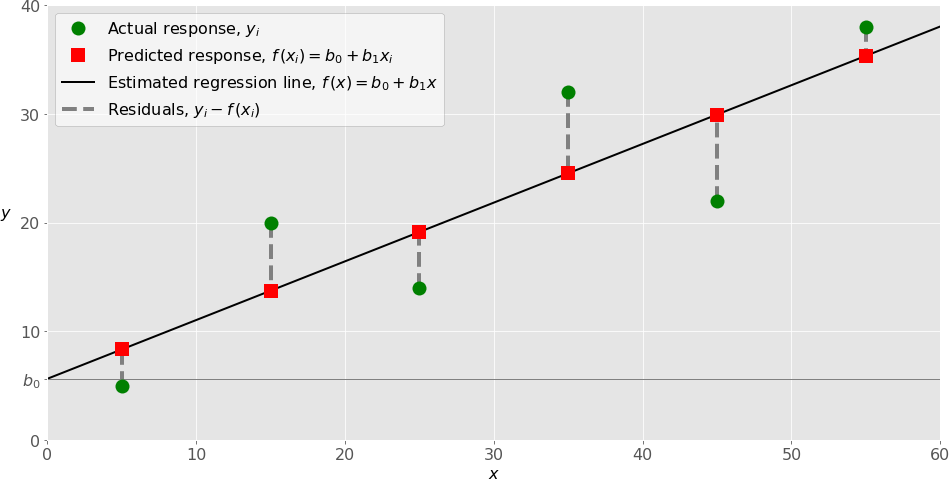
The estimated regression function, represented by the black line, has the equation 𝑓(𝑥) = 𝑏₀ + 𝑏₁𝑥. Your goal is to calculate the optimal values of the predicted weights 𝑏₀ and 𝑏₁ that minimize SSR and determine the estimated regression function.
- The value of 𝑏₀, also called the intercept, shows the point where the estimated regression line crosses the 𝑦 axis. It’s the value of the estimated response 𝑓(𝑥) for 𝑥 = 0.
- The value of 𝑏₁ determines the slope of the estimated regression line.
The vertical dashed grey lines represent the residuals, which can be calculated as 𝑦ᵢ - 𝑓(𝐱ᵢ) = 𝑦ᵢ - 𝑏₀ - 𝑏₁𝑥ᵢ for 𝑖 = 1, …, 𝑛. They’re the distances between the green circles and red squares. When you implement linear regression, you’re actually trying to minimize these distances and make the red squares as close to the predefined green circles as possible.

Python Packages for Linear Regression

NumPy is a fundamental Python scientific package that allows many high-performance operations on single-dimensional and multidimensional arrays. It also offers many mathematical routines.
scikit-learn is a widely used Python library for machine learning, built on top of NumPy and some other packages. It provides the means for preprocessing data, reducing dimensionality, implementing regression, classifying, clustering, and more. Like NumPy, scikit-learn is also open-source.
statsmodels is a powerful Python package for the estimation of statistical models, performing tests, and more.

(venv) $ python -m pip install numpy scikit-learn statsmodels

Simple Linear Regression With scikit-learn

There are five basic steps when you’re implementing linear regression:

Import the packages and classes that you need.
- You’ll use the class sklearn.linear_model.LinearRegression to perform linear and polynomial regression and make predictions accordingly.
Provide data to work with, and eventually do appropriate transformations.
- Input two arrays: the input, x, and the output, y. You should call .reshape() on x because this array must be two-dimensional, or more precisely, it must have one column and as many rows as necessary. That’s exactly what the argument (-1, 1) of .reshape() specifies.
Create a regression model and fit it with existing data.
- Create an instance of the class LinearRegression, which will represent the regression model. You can provide several optional parameters to LinearRegression:
  - fit_intercept is a Boolean that, if True, decides to calculate the intercept 𝑏₀ or, if False, considers it equal to zero. It defaults to True.
  - normalize is a Boolean that, if True, decides to normalize the input variables. It defaults to False, in which case it doesn’t normalize the input variables.
  - copy_X is a Boolean that decides whether to copy (True) or overwrite the input variables (False). It’s True by default.
  - n_jobs is either an integer or None. It represents the number of jobs used in parallel computation. It defaults to None, which usually means one job. -1 means to use all available processors.
- With .fit(), you calculate the optimal values of the weights 𝑏₀ and 𝑏₁, using the existing input and output, x and y, as the arguments. In other words, .fit() fits the model.
Check the results of model fitting to know whether the model is satisfactory.
- When you’re applying .score(), the arguments are also the predictor x and response y, and the return value is 𝑅².
- The attributes of model are .intercept_, which represents the coefficient 𝑏₀, and .coef_, which represents 𝑏₁:
Apply the model for predictions.
- When applying .predict(), you pass the regressor as the argument and get the corresponding predicted response.

import numpy as np
from sklearn.linear_model import LinearRegression
x = np.array([5, 15, 25, 35, 45, 55]).reshape((-1, 1))
y = np.array([5, 20, 14, 32, 22, 38])
model = LinearRegression().fit(x, y)
r_sq = model.score(x, y)
print(f"coefficient of determination: {r_sq}")
print(f"intercept: {model.intercept_}")
print(f"slope: {model.coef_}")
y_pred = model.predict(x)
print(f"predicted response:\n{y_pred}")

Multiple Linear Regression With scikit-learn

You can implement multiple linear regression following the same steps as you would for simple regression. The main difference is that your x array will now have two or more columns.

import numpy as np
from sklearn.linear_model import LinearRegression
x = [
  [0, 1], [5, 1], [15, 2], [25, 5], [35, 11], [45, 15], [55, 34], [60, 35]
]
y = [4, 5, 20, 14, 32, 22, 38, 43]
x, y = np.array(x), np.array(y)
model = LinearRegression().fit(x, y)
r_sq = model.score(x, y)
print(f"coefficient of determination: {r_sq}")
print(f"intercept: {model.intercept_}")
print(f"coefficients: {model.coef_}")
y_pred = model.predict(x)
print(f"predicted response:\n{y_pred}")

Polynomial Regression With scikit-learn

Implementing polynomial regression with scikit-learn is very similar to linear regression. There’s only one extra step: you need to transform the array of inputs to include nonlinear terms such as 𝑥².

The variable transformer refers to an instance of PolynomialFeatures that you can use to transform the input x.

You can provide several optional parameters to PolynomialFeatures:

degree is an integer (2 by default) that represents the degree of the polynomial regression function.
interaction_only is a Boolean (False by default) that decides whether to include only interaction features (True) or all features (False).
include_bias is a Boolean (True by default) that decides whether to include the bias, or intercept, column of 1 values (True) or not (False).

# Step 1: Import packages and classes
import numpy as np
from sklearn.linear_model import LinearRegression
from sklearn.preprocessing import PolynomialFeatures

# Step 2a: Provide data
x = [
  [0, 1], [5, 1], [15, 2], [25, 5], [35, 11], [45, 15], [55, 34], [60, 35]
]
y = [4, 5, 20, 14, 32, 22, 38, 43]
x, y = np.array(x), np.array(y)

# Step 2b: Transform input data
x_ = PolynomialFeatures(degree=2, include_bias=False).fit_transform(x)

# Step 3: Create a model and fit it
model = LinearRegression().fit(x_, y)

# Step 4: Get results
r_sq = model.score(x_, y)
intercept, coefficients = model.intercept_, model.coef_

# Step 5: Predict response
y_pred = model.predict(x_)