reading-notes

Trees

Common Terminology

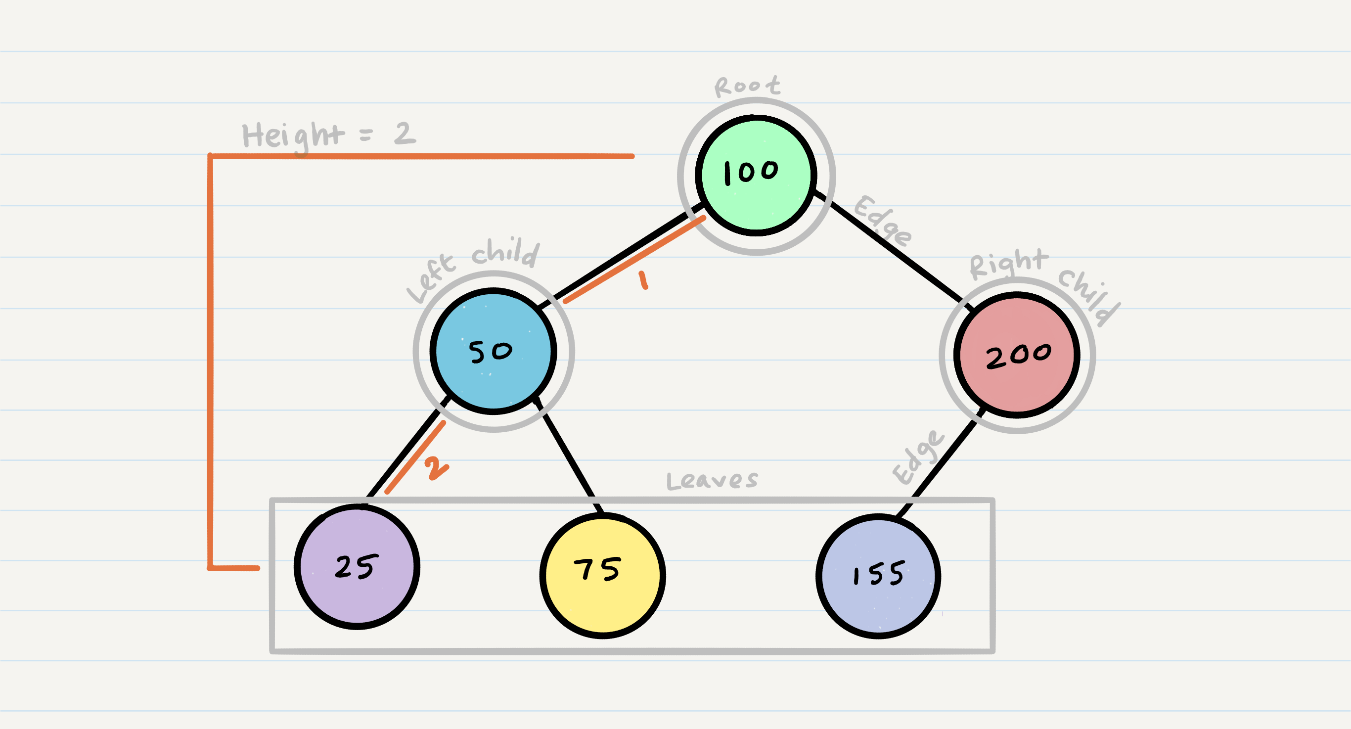
Node - A Tree node is a component which may contain its own values, and references to other nodes
Root - The root is the node at the beginning of the tree
‘k’ - A number that specifies the maximum number of children any node may have in a k-ary tree. In a binary tree, k = 2.
Left - A reference to one child node, in a binary tree
Right - A reference to the other child node, in a binary tree
Edge - The edge in a tree is the link between a parent and child node
Leaf - A leaf is a node that does not have any children
Height - The height of a tree is the number of edges from the root to the furthest leaf

Trees

Traversals

An important aspect of trees is how to traverse them. Traversing a tree allows us to search for a node, print out the contents of a tree, and much more! There are two categories of traversals when it comes to trees:

Depth First - where we prioritize going through the depth (height) of the tree first. There are multiple ways to carry out depth first traversal, and each method changes the order in which we search/print the root. The most common way to traverse through a tree is to use recursion. With these traversals, we rely on the call stack to navigate back up the tree when we have reached the end of a sub-path.Here are three methods for depth first traversal:
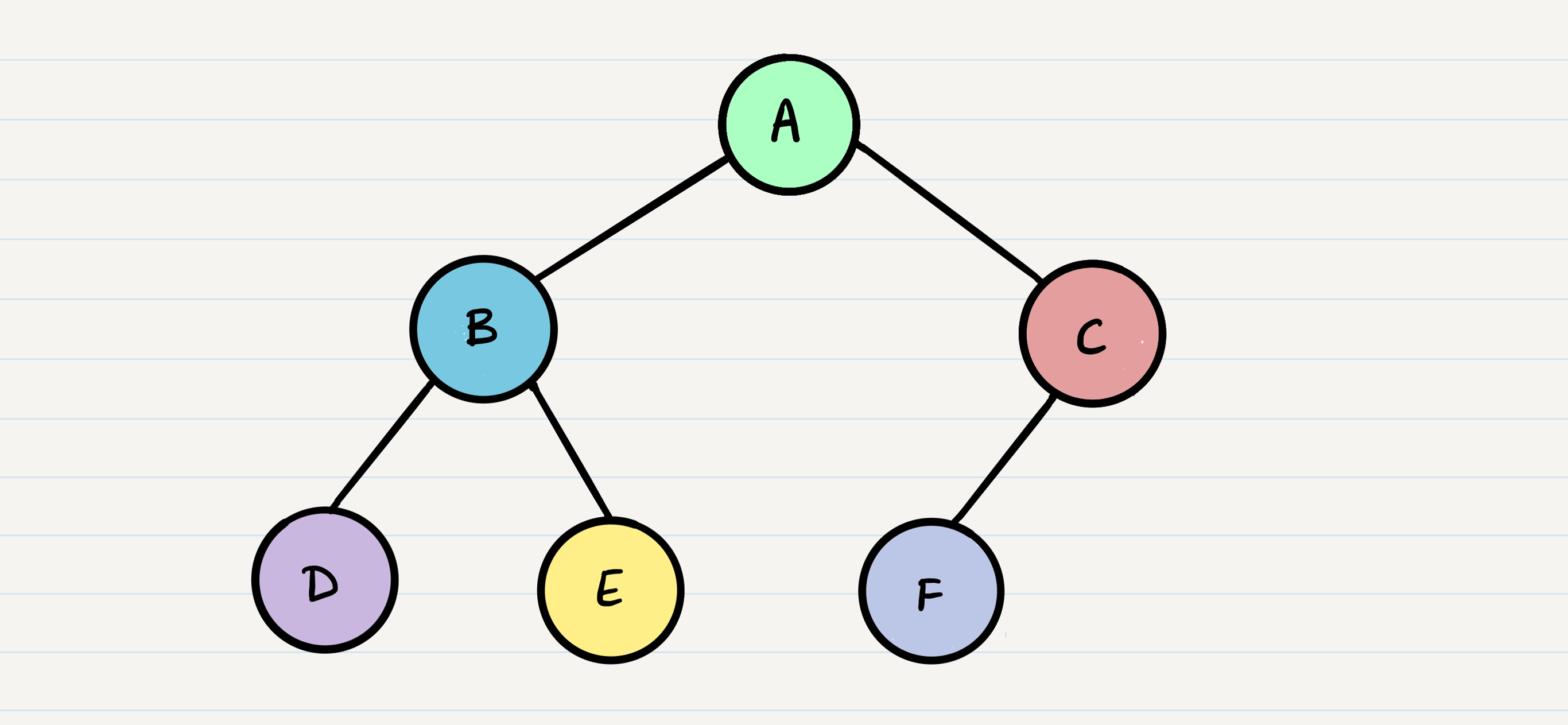
- Pre-order: root >> left >> right -> A, B, D, E, C, F
```
ALGORITHM preOrder(root)
// INPUT <-- root node
// OUTPUT <-- pre-order output of tree node's values

OUTPUT <-- root.value

if root.left is not Null
    preOrder(root.left)

if root.right is not NULL
    preOrder(root.right)
```
- In-order: left >> root >> right -> D, B, E, A, F, C
```
ALGORITHM inOrder(root)
// INPUT <-- root node
// OUTPUT <-- in-order output of tree node's values

if root.left is not NULL
    inOrder(root.left)

OUTPUT <-- root.value

if root.right is not NULL
    inOrder(root.right)
```
- Post-order: left >> right >> root -> ` D, E, B, F, C, A`
```
ALGORITHM postOrder(root)
// INPUT <-- root node
// OUTPUT <-- post-order output of tree node's values

if root.left is not NULL
    postOrder(root.left)

if root.right is not NULL
    postOrder(root.right)

OUTPUT <-- root.value
```
  Notice the similarities between the three different traversals above. The biggest difference between each of the traversals is when you are looking at the root node.

Depth First

Breadth First - iterates through the tree by going through each level of the tree node-by-node. Traditionally, breadth first traversal uses a queue (instead of the call stack via recursion) to traverse the width/breadth of the tree. Let’s break down the process:

Given our starting tree shown above, let’s start by putting the root into the queue.
Now that we have one node in our queue, we can dequeue it and use that node in our code.
From our dequeued node A, we can enqueue the left and right child (in that order).
This leaves us with B as the new front of our queue. We can then repeat the process we did with A: Dequeue the front node, enqueue that node’s left and right nodes, and move to the next new front of the queue.
Now our front is C, so we repeat the dequeue + enqueue children process:
And we continue onwards. When we reach a node that doesn’t have any children, we just dequeue it without any further enqueue.

ALGORITHM breadthFirst(root)
// INPUT  <-- root node
// OUTPUT <-- front node of queue to console

  Queue breadth <-- new Queue()
  breadth.enqueue(root)

  while ! breadth.is_empty()
    node front = breadth.dequeue()
    OUTPUT <-- front.value

    if front.left is not NULL
      breadth.enqueue(front.left)

    if front.right is not NULL
      breadth.enqueue(front.right)

Adding a Node

Because there are no structural rules for where nodes are “supposed to go” in a binary tree, it really doesn’t matter where a new node gets placed.

One strategy for adding a new node to a binary tree is to fill all “child” spots from the top down. To do so, we would leverage the use of breadth first traversal. During the traversal, we find the first node that does not have all its children filled, and insert the new node as a child. We fill the child slots from left to right.

In the event you would like to have a node placed in a specific location, you need to reference both the new node to create, and the parent node which the child is attached to.

Big O - Adding a Node

The Big O time complexity for inserting a new node is O(n). Searching for a specific node will also be O(n). Because of the lack of organizational structure in a Binary Tree, the worst case for most operations will involve traversing the entire tree. If we assume that a tree has n nodes, then in the worst case we will have to look at n items, hence the O(n) complexity.

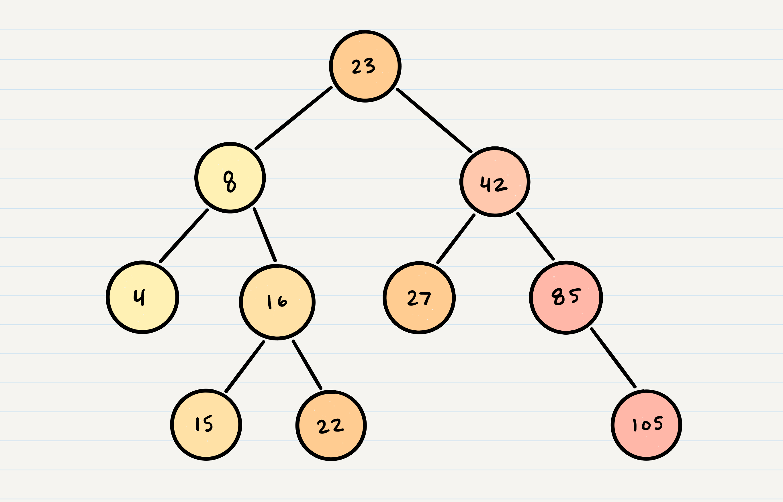
The Big O space complexity for a node insertion using breadth first insertion will be O(w), where w is the largest width of the tree. For example, in the above tree, w is 4.

A “perfect” binary tree is one where every non-leaf node has exactly two children. The maximum width for a perfect binary tree, is 2^(h-1), where h is the height of the tree. Height can be calculated as log n, where n is the number of nodes.

Binary Search Trees

A Binary Search Tree (BST) is a type of tree that does have some structure attached to it. In a BST, nodes are organized in a manner where all values that are smaller than the root are placed to the left, and all values that are larger than the root are placed to the right.

BST

Searching a BST

Searching a BST can be done quickly, because all you do is compare the node you are searching for against the root of the tree or sub-tree. If the value is smaller, you only traverse the left side. If the value is larger, you only traverse the right side.

Let’s say we are searching 15. We start by comparing the value 15 to the value of the root, 23.
15 < 23, so we traverse the left side of the tree. We then treat 8 as our new “root” to compare against.
15 > 8, so we traverse the right side. 16 is our new root.
15 < 16, so we traverse the left side. 15 is our new root and also a match with what we were searching for.

Search BST

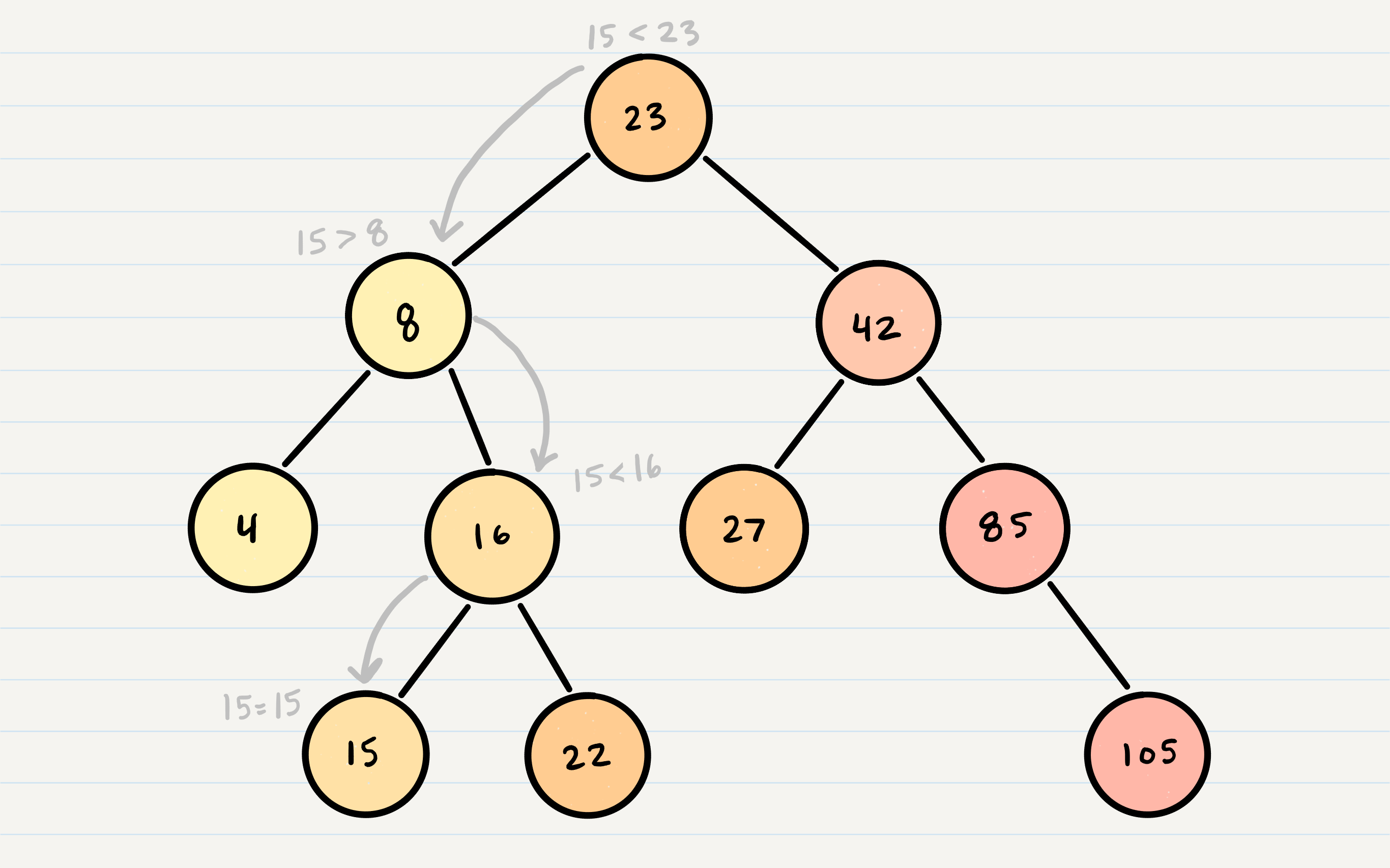
The best way to approach a BST search is with a while loop. We cycle through the while loop until we hit a leaf, or until we reach a match with what we’re searching for.

Big O - Searching a BST

The Big O time complexity of a Binary Search Tree’s insertion and search operations is O(h), or O(height). In the worst case, we will have to search all the way down to a leaf, which will require searching through as many nodes as the tree is tall. In a balanced (or “perfect”) tree, the height of the tree is log(n). In an unbalanced tree, the worst case height of the tree is n.

The Big O space complexity of a BST search would be O(1). During a search, we are not allocating any additional space.

Source: https://codefellows.github.io/common_curriculum/data_structures_and_algorithms/Code_401/class-15/resources/Trees.html