reading-notes
Module 1 - Create machine learning models
Train and evaluate clustering models
What is clustering?
Clustering is a form of unsupervised machine learning in which observations are grouped into clusters based on similarities in their data values, or features. This kind of machine learning is considered unsupervised because it does not make use of previously known label values to train a model; in a clustering model, the label is the cluster to which the observation is assigned, based purely on its features.
Let’s take a look at a dataset that contains measurements of different species of wheat seed. The dataset contains six data points (or features) for each instance (observation) of a seed. So you could interpret these as coordinates that describe each instance’s location in six-dimensional space.
Six-dimensional space is difficult to visualize in a three-dimensional world, or on a two-dimensional plot; so we’ll take advantage of a mathematical technique called Principal Component Analysis (PCA) to analyze the relationships between the features and summarize each observation as coordinates for two principal components - in other words, we’ll translate the six-dimensional feature values into two-dimensional coordinates.
  import pandas as pd
  from sklearn.preprocessing import MinMaxScaler
  from sklearn.decomposition import PCA
  import matplotlib.pyplot as plt
  %matplotlib inline

  # load the training dataset
  !wget https://raw.githubusercontent.com/MicrosoftDocs/mslearn-introduction-to-machine-learning/main/Data/ml-basics/seeds.csv
  data = pd.read_csv('seeds.csv')

  # Normalize the numeric features so they're on the same scale
  scaled_features = MinMaxScaler().fit_transform(features[data.columns[0:6]])

  # Get two principal components
  pca = PCA(n_components=2).fit(scaled_features)
  features_2d = pca.transform(scaled_features)
  features_2d[0:10]

  plt.scatter(features_2d[:,0],features_2d[:,1])
  plt.xlabel('Dimension 1')
  plt.ylabel('Dimension 2')
  plt.title('Data')
  plt.show()
We can create a series of clustering models with an incrementing number of clusters and measure how tightly the data points are grouped within each cluster. A metric often used to measure this tightness is the within cluster sum of squares (WCSS), with lower values meaning that the data points are closer. You can then plot the WCSS for each model.
  #importing the libraries
  import numpy as np
  import matplotlib.pyplot as plt
  from sklearn.cluster import KMeans
  %matplotlib inline

  # Create 10 models with 1 to 10 clusters
  wcss = []
  for i in range(1, 11):
      kmeans = KMeans(n_clusters = i)
      # Fit the data points
      kmeans.fit(features.values)
      # Get the WCSS (inertia) value
      wcss.append(kmeans.inertia_)

  #Plot the WCSS values onto a line graph
  plt.plot(range(1, 11), wcss)
  plt.title('WCSS by Clusters')
  plt.xlabel('Number of clusters')
  plt.ylabel('WCSS')
  plt.show()
The plot shows a large reduction in WCSS (so greater tightness) as the number of clusters increases from one to two, and a further noticeable reduction from two to three clusters. After that, the reduction is less pronounced, resulting in an “elbow” in the chart at around three clusters. This is a good indication that there are two to three reasonably well separated clusters of data points.
Training a clustering model
There are multiple algorithms you can use for clustering. One of the most commonly used algorithms is K-Means clustering* that, in its simplest form, consists of the following steps:
- The feature values are vectorized to define n-dimensional coordinates (where
nis the number of features). - You decide how many clusters you want to use to group, and call this value
k. Thenkpoints are plotted at random coordinates. These points will ultimately be the center points for each cluster, so they’re referred to as centroids. - Each data point is assigned to its nearest centroid.
- Each centroid is moved to the center of the data points assigned to it based on the mean distance between the points.
- After moving the centroid, the data points may now be closer to a different centroid, so the data points are reassigned to clusters based on the new closest centroid.
- The centroid movement and cluster reallocation steps are repeated until the clusters become stable or a pre-determined maximum number of iterations is reached.

Hierarchical clustering is another type of clustering algorithm in which clusters themselves belong to a larger group, which belong to even larger groups, and so on. The result is that data points can be clusters in differing degrees of precision: with a large number of very small and precise groups, or a small number of larger groups.
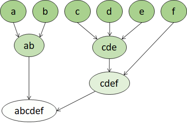
Hierarchical clustering is useful for not only breaking data into groups, but understanding the relationships between these groups. A major advantage of hierarchical clustering is that it does not require the number of clusters to be defined in advance, and can sometimes provide more interpretable results than non-hierarchical approaches. The major drawback is that these approaches can take much longer to compute than simpler approaches and sometimes are not suitable for large datasets.
Hierarchical clustering creates clusters by either a divisive method or agglomerative method. The divisive method is a “top down” approach starting with the entire dataset and then finding partitions in a stepwise manner. Agglomerative clustering is a “bottom up” approach.
Clustering examples
Using the previous example, we can use K-Means on our seeds data with a K value of 3.
  from sklearn.cluster import KMeans
  import matplotlib.pyplot as plt
  %matplotlib inline

  # Create a model based on 3 centroids
  model = KMeans(n_clusters=3, init='k-means++', n_init=100, max_iter=1000)
  # Fit to the data and predict the cluster assignments for each data point
  km_clusters = model.fit_predict(features.values)
  # View the cluster assignments
  km_clusters

  def plot_clusters(samples, clusters):
      col_dic = {0:'blue',1:'green',2:'orange'}
      mrk_dic = {0:'*',1:'x',2:'+'}
      colors = [col_dic[x] for x in clusters]
      markers = [mrk_dic[x] for x in clusters]
      for sample in range(len(clusters)):
          plt.scatter(samples[sample][0], samples[sample][1], color = colors[sample], marker=markers[sample], s=100)
      plt.xlabel('Dimension 1')
      plt.ylabel('Dimension 2')
      plt.title('Assignments')
      plt.show()

  plot_clusters(features_2d, km_clusters)
Let’s see an example of clustering the seeds data using an agglomerative clustering algorithm.
  from sklearn.cluster import AgglomerativeClustering
  import matplotlib.pyplot as plt
  %matplotlib inline

  agg_model = AgglomerativeClustering(n_clusters=3)
  agg_clusters = agg_model.fit_predict(features.values)
  agg_clusters

  def plot_clusters(samples, clusters):
      col_dic = {0:'blue',1:'green',2:'orange'}
      mrk_dic = {0:'*',1:'x',2:'+'}
      colors = [col_dic[x] for x in clusters]
      markers = [mrk_dic[x] for x in clusters]
      for sample in range(len(clusters)):
          plt.scatter(samples[sample][0], samples[sample][1], color = colors[sample], marker=markers[sample], s=100)
      plt.xlabel('Dimension 1')
      plt.ylabel('Dimension 2')
      plt.title('Assignments')
      plt.show()

  plot_clusters(features_2d, agg_clusters)
Summary
In this module, you learned how clustering can be used to create unsupervised machine learning models that group data observations into clusters. You then used the scikit-learn framework in Python to train a clustering model.
Source: Microsoft Learn