reading-notes

Module 1 - Create machine learning models

Train and evaluate deep learning models

Deep learning is an advanced form of machine learning that tries to emulate the way the human brain learns using artificial neural networks that process numeric inputs rather than electrochemical stimuli.

The incoming nerve connections are replaced by numeric inputs that are typically identified as x. When there’s more than one input value, x is considered a vector with elements named x1, x2, and so on.

Associated with each x value is a weight (w), which is used to strengthen or weaken the effect of the x value to simulate learning. Additionally, a bias (b) input is added to enable fine-grained control over the network. During the training process, the w and b values will be adjusted to tune the network so that it “learns” to produce correct outputs.

The neuron itself encapsulates a function that calculates a weighted sum of x, w, and b. This function is in turn enclosed in an activation function that constrains the result (often to a value between 0 and 1) to determine whether or not the neuron passes an output onto the next layer of neurons in the network.

Deep neural network concepts

The deep neural network (DNN) model for the classifier consists of multiple layers of artificial neurons. An example would be classifying a sample as one of three penguin species based on 4 attributes. In this case, there are four layers:

• An input layer with a neuron for each expected input (x) value.
• Two so-called hidden layers, each containing five neurons.
• An output layer containing three neurons - one for each class probability (y) value to be predicted by the model.

You can decide how many hidden layers you want to include and how many neurons are in each of them; but you have no control over the input and output values for these layers - these are determined by the model training process.

Because of the layered architecture of the network, this kind of model is sometimes referred to as a multilayer perceptron. Additionally, notice that all neurons in the input and hidden layers are connected to all neurons in the subsequent layers - this is an example of a fully connected network.

The training process for a deep neural network consists of multiple iterations, called epochs. For the first epoch, you start by assigning random initialization values for the weight (w) and bias (b) values. Then the process is as follows:

1. Features for data observations with known label values are submitted to the input layer. Generally, these observations are grouped into batches (often referred to as mini-batches).
2. The neurons then apply their function, and if activated, pass the result onto the next layer until the output layer produces a prediction.
3. The prediction is compared to the actual known value, and the amount of variance between the predicted and true values (which we call the loss) is calculated.
4. Based on the results, revised values for the weights and bias values are calculated to reduce the loss, and these adjustments are back-propagated to the neurons in the network layers.
5. The next epoch repeats the batch training forward pass with the revised weight and bias values, hopefully improving the accuracy of the model (by reducing the loss).

An optimizer is an algorithm used to minimize the loss function of a neural network. It does this by updating the weights of the network based on the gradients of the loss function with respect to the weights. There are many different optimizers available, such as Stochastic Gradient Descent (SGD), Adam, Adagrad, and RMSprop, each with their own strengths and weaknesses.

The learning rate is a hyperparameter that determines how quickly the weights of the network are updated during training. It controls the step size in the weight space that the optimizer takes in each iteration. If the learning rate is too high, the optimizer may overshoot the minimum of the loss function and fail to converge, while if it is too low, the optimization may be too slow and require more time to converge.

In practice, finding the optimal learning rate for a given optimizer can be challenging, and a common approach is to use a learning rate schedule or adaptive learning rate methods, such as cosine annealing or learning rate decay, to gradually reduce the learning rate during training to help the optimizer converge to a good solution.

---

Convolutional neural networks

Machine learning models that work with images are the foundation for an area artificial intelligence called computer vision, and deep learning techniques have been responsible for driving amazing advances in this area over recent years.

Convolutional neural network (CNN) typically works by extracting features from images, and then feeding those features into a fully connected neural network to generate a prediction. The feature extraction layers in the network have the effect of reducing the number of features from the potentially huge array of individual pixel values to a smaller feature set that supports label prediction.

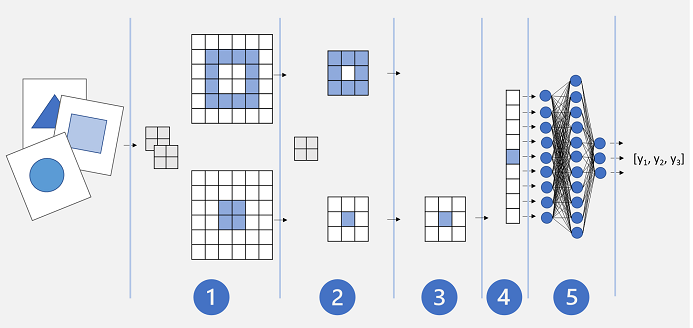
CNNs consist of multiple layers, each performing a specific task in extracting features or predicting labels:

• Convolution layers - Extracts important features in images. A convolutional layer works by applying a filter to images which is defined by a kernel that consists of a matrix of weight values (like a 3x3 filter). To apply the filter, you “overlay” it on an image and calculate a weighted sum of the corresponding image pixel values under the filter kernel. The result is then assigned to the center cell of an equivalent 3x3 patch in a new matrix of values that is the same size as the image. The resulting matrix is a feature map of feature values that can be used to train a machine learning model.
• Pooling layers - After extracting feature values from images, pooling (or downsampling) layers are used to reduce the number of feature values while retaining the key differentiating features that have been extracted. One of the most common kinds of pooling is max pooling in which a filter is applied to the image, and only the maximum pixel value within the filter area is retained. The pooling kernel is convolved across the feature map, retaining only the highest pixel value in each position.
• Dropping layers - One of the most difficult challenges in a CNN is the avoidance of overfitting, where the resulting model performs well with the training data but doesn’t generalize well to new data on which it wasn’t trained. One technique you can use to mitigate overfitting is to include layers in which the training process randomly eliminates (or “drops”) feature maps to ensure that the model doesn’t learn to be over-dependent on the training images. Other techniques you can use to mitigate overfitting include randomly flipping, mirroring, or skewing the training images to generate data that varies between training epochs.
• Flattening layers - After using convolutional and pooling layers to extract the salient features in the images, the resulting feature maps are multidimensional arrays of pixel values. A flattening layer is used to flatten the feature maps into a vector of values that can be used as input to a fully connected layer.
• Fully connected layers - Usually, a CNN ends with a fully connected network in which the feature values are passed into an input layer, through one or more hidden layers, and generate predicted values in an output layer.

Transfer learning

A Convolutional Neural Network (CNN) for image classification is typically composed of multiple layers that extract features, and then use a final fully connected layer to classify images based on these features.

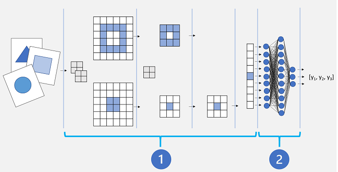
Conceptually, this neural network consists of two distinct sets of layers:

1. A set of layers from the base model that perform feature extraction.
2. A fully connected layer that takes the extracted features and uses them for class prediction.

The feature extraction layers apply convolutional filters and pooling to emphasize edges, corners, and other patterns in the images that can be used to differentiate them, and in theory should work for any set of images with the same dimensions as the input layer of the network. The prediction layer maps the features to a set of outputs that represent probabilities for each class label you want to use to classify the images.

By separating the network into these types of layers, we can take the feature extraction layers from a model that has already been trained and append one or more layers to use the extracted features for prediction of the appropriate class labels for your images. This approach enables you to keep the pre-trained weights for the feature extraction layers, which means you only need to train the prediction layers you have added.

---

PyTorch and TensorFlow

PyTorch and TensorFlow are two of the most popular deep learning frameworks used for building and training neural networks.

• PyTorch is an open-source machine learning library developed by Facebook’s AI research team. It is a dynamic computational graph framework, meaning that it allows for efficient model building and training using dynamic graphs that can be modified on the fly. PyTorch provides a high-level interface for building neural networks, and it has become a popular choice for researchers and developers due to its ease of use and flexibility. PyTorch supports both CPU and GPU computations and offers a variety of modules and functions for building various types of neural networks, including Convolutional Neural Networks (CNNs), Recurrent Neural Networks (RNNs), and Transformers.
• TensorFlow is another open-source machine learning library developed by Google. It is a static computational graph framework, meaning that it requires the user to define the graph structure before training the model. TensorFlow provides a wide range of tools and features for building and training neural networks, including distributed computing capabilities, visualization tools, and support for both CPU and GPU computations. TensorFlow has a large community of users and contributors, making it a popular choice for both research and industry applications.

Both PyTorch and TensorFlow have their own strengths and weaknesses, and the choice between the two often depends on the specific use case and personal preferences. While PyTorch offers dynamic graphs and an intuitive interface, TensorFlow offers more advanced features and a wider range of tools for distributed computing and deployment. Ultimately, both frameworks are powerful tools for building and training deep learning models.

Summary

In this module you learned about the fundamental principles of deep learning, and how to create deep neural network models using PyTorch or Tensorflow. You also explored the use of convolutional neural networks to create image classification models.

Source: Microsoft Learn